Input for BayesianNetworkRegression.jl

The function Fit! within BayesianNetworkRegression.jl is the main method to estimate the relationships between the edges of the microbiome network (covariates) and the variable of interest (response).

There are two alternatives for the network input data:

1. A vector of matrices, where each item in the vector (of length $n$, where $n$ is the sample size) is an $V \times V$ (where $V$ is the number of microbes in each sample) adjacency matrix describing the microbiome network. All adjacency matrices must be the same size.
2. A $n \times \frac{V(V-1)}{2}$ matrix, where each row in the matrix is the upper triangle of the adjacency matrix describing the network for that sample.

Note that the package does not assume any specific inference procedure for the estimation of the adjacency matrices (and thus, of the microbiome networks). This means that the microbiome networks can be obtained using the user's preferred methodology and simply input them into the package as described below.

Tutorial data: Adjacency matrices

Suppose that you design an experiment with $n$ different samples, and for each sample, you estimate a microbial network for $V$ microbes and a measured phenotype.

The $n$ microbial networks can be stored as $n$ adjacency matrices. We have a toy example where we stored the adjacency matrices as a JLD2 file with the JLD2.jl package.

You have two files:

1. vector_networks.jld2 contains a vector of adjacency matrices and
2. vector_response.jld2 contains a vector of responses (real numbers).

You can access the example files for the networks here and for the responses here

To load the data and view an example in julia do the following:

using BayesianNetworkRegression
using JLD2
cd(joinpath(dirname(pathof(BayesianNetworkRegression)), "..","examples"))

vector_networks = JLD2.load("vector_networks.jld2")
vector_response = JLD2.load("vector_response.jld2")

vector_networks["networks"][1] # shows the first adjancency matrix
vector_response["response"] # shows all responses

X_a = vector_networks["networks"]
y_a = vector_response["response"]

We will use the X_a and y_a objects in the Fit! function in the next section.

Reading adjacency matrices from csv files

Most of the times, researchers will have stored the adjacency matrices as csv files (rather than JLD files as in the previous section). In this example, you have 100 adjacency matrices stored as data1.csv,...,data100.csv, as well as a csv file for the 100-dimension vector of the responses: responses.csv.

using BayesianNetworkRegression
using CSV, Tables, DataFrames

vector_response = CSV.read("responses.csv", DataFrame)

vector_networks = Matrix{Float64}[]
for i in 1:100
dat = CSV.read(string("data",i,".csv"),DataFrame)
push!(vector_networks, Matrix(dat))
end

X_a = vector_networks
y_a = vector_response[:,1]

We will use the X_a and y_a objects in the Fit! function in the next section.

Tutorial data: Vectorized adjacency matrices

Suppose that you already converted each adjacency matrix into a vector corresponding to its upper triangle (see image below).

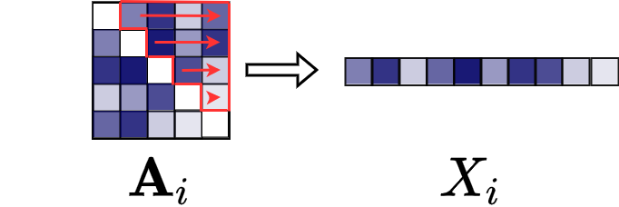
That is, you have a file with $n$ rows and $\frac{V(V-1)}{2} + 1$ columns. For each row, the first $\frac{V(V-1)}{2}$ columns describe the upper triangle of an adjacency matrix and the last column gives the response variable.

You can access the example file of input networks (and response) here.

Do not copy-paste into a "smart" text-editor. Instead, save the file directly into your working directory using "save link as" or "download linked file as". This file contains 100 adjacency matrices and corresponding responses.

To load the data and view an example in julia do the following:

using CSV, DataFrames
cd(joinpath(dirname(pathof(BayesianNetworkRegression)), "..","examples"))

dat = DataFrame(CSV.File("matrix_networks.csv"))
X_v = Matrix(dat[:,1:435])
y_v = dat[:,436]

We will use the X_v and y_v objects in the Fit! function in the next section.