Estimating phylogenetic networks with SNaQ
To run SNaQ, you need
- data extracted from sequence alignments:
- a list of estimated unrooted gene trees, or
- a table of concordance factors (CF) (e.g. from BUCKy)
- a starting topology (e.g. from Quartet MaxCut or ASTRAL, or RAxML tree from a single gene…)
In the analysis folder, we have:
- starting topology in
nexus.QMC.tre - table of concordance factors in
nexus.CFs.csv
We move into the analysis folder and start a julia session:
cd analysis
julia
Note that we do not need to run this inside the Docker container anymore. We can run this locally as long as Julia is installed.
Loading the Julia packages in Julia:
using PhyloNetworks
using SNaQ
using PhyloPlots
1. Read the CF table into Julia:
buckyCF = readtableCF("nexus.CFs.csv")
For the commands to read estimated gene trees, see here.
2. Read the starting population tree into Julia:
tre = readnewick("nexus.QMC.tre")
3. Estimate the best network for a number of hybridizations
Estimate the best network from BUCKy’s quartet CF and hmax number of hybridizations:
net1 = snaq!(tre, buckyCF, hmax=1, runs=1, filename="net1_snaq", seed=456, ftolRel=1.0e-4, ftolAbs=1.0e-4,liktolAbs = 1.0e-4)
The options we are using are:
hmax=1: maximum one hybridization eventruns=1: number of runs for the optimization; set to 1 to make the run fast, but you want to do at leastruns=10(which is the default) for your real analysisfilename="net1_snaq": rootname for the output files (described below)seed=456: random seed to replicate the analysisftolRel=1.0e-4, ftolAbs=1.0e-4,liktolAbs = 1.0e-4: optimization tolerance values chosen so that the run is fast. For your analyses, you do not need to specify these quantities and can simply use the defaults
The following output is printed to the screen:
optimization of topology, BL and inheritance probabilities in SNaQ.jl using:
hmax = 1,
tolerance parameters: ftolRel=0.0001, ftolAbs=0.0001,
xtolAbs=0.001, xtolRel=0.01.
max number of failed proposals = 75, liktolAbs = 0.0001.
rootname for files: net1_snaq
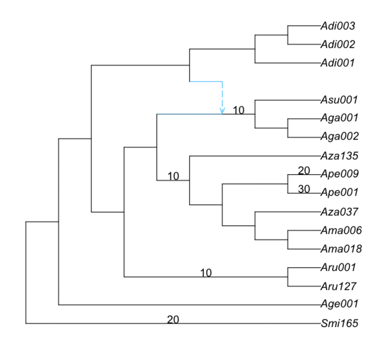
BEGIN: 1 runs on starting tree (Adi003,Adi002,(Adi001,((Smi165,Age001):0.11282763783172885,((Aru001,Aru127):1.8895892722315206,(((((Ama018,Ama006):0.635979116918197,Aza037):0.2064967739309278,(Ape001,Ape009):0.7567729870351637):0.17709162771363504,Aza135):1.3242277867359862,((Aga002,Aga001):1.1662225201998988,Asu001):1.33643060185584):0.10642736789559729):0.45657761568828575):2.424105745425032):0.1638513742450063);
2025-05-20 15:51:6.718
seed: 456 for run 1, 2025-05-20 15:51:8.268
best network and networks with different hybrid/gene flow directions printed to .networks file
MaxNet is ((Adi001,(((Smi165,Age001):0.10909139515055954,((Aru001,Aru127):1.783553809432207,(((((Ama018,Ama006):0.6686980253651718,Aza037):0.19099507776876928,(Ape001,Ape009):0.754921262227867):0.15053133922303902,Aza135):1.1427622517130929,((Asu001,(Aga002,Aga001):0.9081531659227717):0.48236561520817717)#H17:2.0594381934607306::0.8210853726908922):0.18471450412843127):0.5158573560102714):0.22659449745358853,#H17:0.697544251960922::0.17891462730910784):2.1586763301439107):0.1426954054706382,Adi003,Adi002);
with -loglik 815.1786591571492
HybridNetwork, Semidirected Network
32 edges
32 nodes: 16 tips, 1 hybrid nodes, 15 internal tree nodes.
tip labels: Adi003, Adi002, Adi001, Smi165, ...
((Adi001,(((Smi165,Age001):0.109,((Aru001,Aru127):1.784,(((((Ama018,Ama006):0.669,Aza037):0.191,(Ape001,Ape009):0.755):0.151,Aza135):1.143,((Asu001,(Aga002,Aga001):0.908):0.482)#H17:2.059::0.821):0.185):0.516):0.227,#H17:0.698::0.179):2.159):0.143,Adi003,Adi002);
To use multiple threads while running SNaQ, see here.
You should increase the number of hybridizations sequentially:
hmax=0,1,2,..., and use the best network at h-1 as starting
point to estimate the best network at h.
4. Overview of the output files
The estimated network is in the net1_snaq.out file which also has the running time: 2082.5 seconds (~35 minutes) in my computer:
% less analysis/net1_snaq.out

((Adi001,(((Smi165,Age001):0.10909139515055954,((Aru001,Aru127):1.783553809432207,(((((Ama018,Ama006):0.6686980253651718,Aza037):0.19099507776876928,(Ape001,Ape009):0.754921262227867):0.15053133922303902,Aza135):1.1427622517130929,((Asu001,(Aga002,Aga001):0.9081531659227717):0.48236561520817717)#H17:2.0594381934607306::0.8210853726908922):0.18471450412843127):0.5158573560102714):0.22659449745358853,#H17:0.697544251960922::0.17891462730910784):2.1586763301439107):0.1426954054706382,Adi003,Adi002); -Ploglik = 815.1786591571492
 Dendroscope: ((Adi001,(((Smi165,Age001):0.10909139515055954,((Aru001,Aru127):1.783553809432207,(((((Ama018,Ama006):0.6686980253651718,Aza037):0.19099507776876928,(Ape001,Ape009):0.754921262227867):0.15053133922303902,Aza135):1.1427622517130929,((Asu001,(Aga002,Aga001):0.9081531659227717):0.48236561520817717)#H17:2.0594381934607306):0.18471450412843127):0.5158573560102714):0.22659449745358853,#H17:0.697544251960922):2.1586763301439107):0.1426954054706382,Adi003,Adi002);
 Elapsed time: 2082.5 seconds, 1 attempted runs
-------
List of estimated networks for all runs (sorted by log-pseudolik; the smaller, the better):
 ((Adi001,(((Smi165,Age001):0.10909139515055954,((Aru001,Aru127):1.783553809432207,(((((Ama018,Ama006):0.6686980253651718,Aza037):0.19099507776876928,(Ape001,Ape009):0.754921262227867):0.15053133922303902,Aza135):1.1427622517130929,((Asu001,(Aga002,Aga001):0.9081531659227717):0.48236561520817717)#H17:2.0594381934607306::0.8210853726908922):0.18471450412843127):0.5158573560102714):0.22659449745358853,#H17:0.697544251960922::0.17891462730910784):2.1586763301439107):0.1426954054706382,Adi003,Adi002);, with -loglik 815.1786591571492
-------
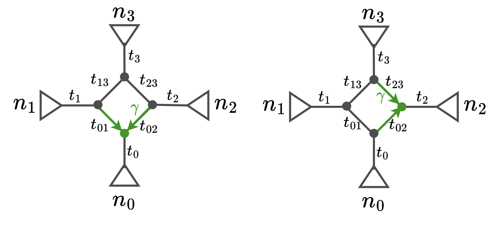
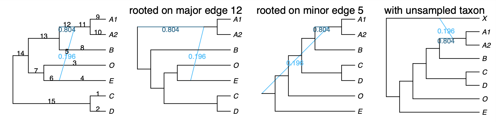
The net1_snaq.networks file contains multiple candidate networks that are obtained by rotating the position of the hybrid node in the hybridization cycle. For example, the figure below shows a hybridization cycle with 4 nodes and two positions for the hybrid node.
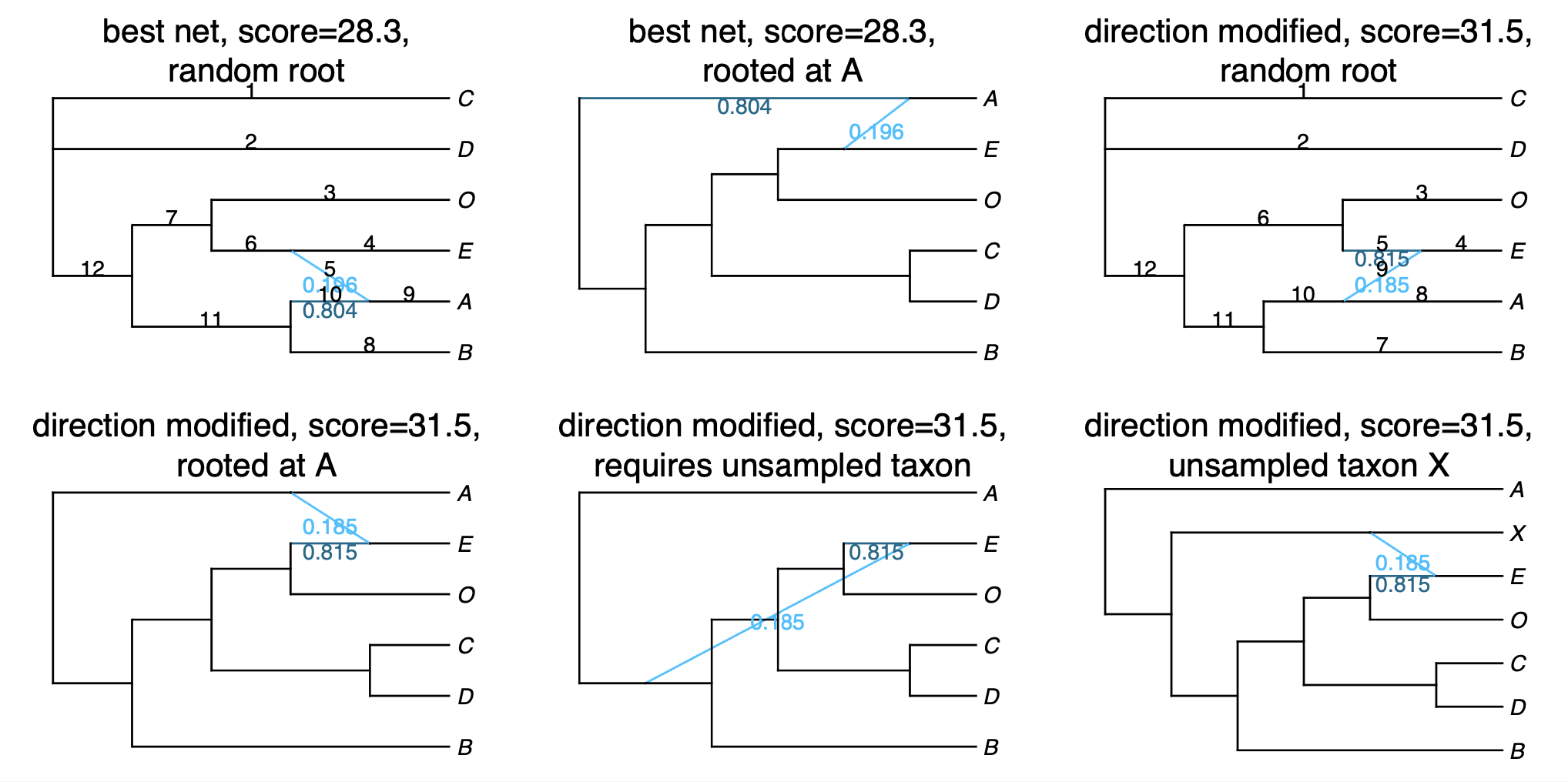
This .networks file exists so that you can check if a different placement of the hybrid node in the cycle makes more sense biologically, or when you cannot root your network on your outgroup because of the position of the hybrid node. Make sure to check the pseudolikelihood score of the candidate networks so that you select one that has comparable pseudolik score to the best network (see an example below).
The files net1_snaq.log and net1_snaq.err contain information about the runs and possible errors, and are only useful if you get an error from SNaQ and want to report it as a GitHub issue.
5. Plot the estimated network
If your snaq process has not finished, and you want to continue with the tutorial, you can read the output file with:
net1 = readnewick("net1_snaq.out")
Recall that the produced network is semi-directed, not rooted, so we need to root at the outgroup:
rootatnode!(net1, "Smi165")
If you get an error when trying to root at your outgroup, make sure to check the .networks file for alternative networks that could have a similar pseudolik score.
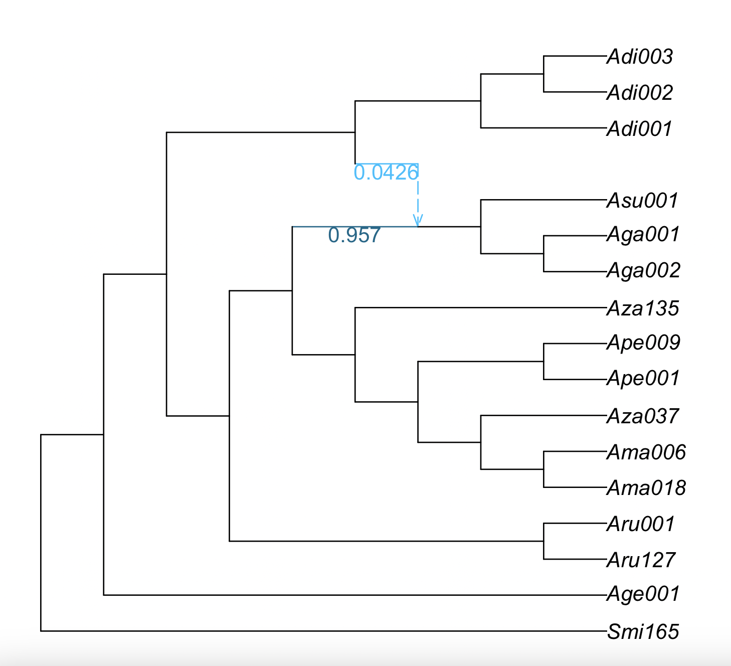
Now, we will plot the estimated networks:
plot(net1, showgamma=true);
If a plot window didn’t pop up, an alternative is to save the plot as a pdf and open it outside of julia:
using RCall
R"pdf"("plot-net1.pdf", width=6, height=6);
plot(net1);
R"dev.off()";
SNaQ can infer hybridizations with extinct or unsampled taxa (ghost lineages). Thus, keep this in mind when interpreting the hybridization event, especially if the hybridization event appears to be connecting an ancestral lineage with a more recent one.
Bootstrapping
You need as input:
- data from sequence alignment that capture uncertainty:
- credibility intervals for quartet concordance factors, from TICR
- bootstrap gene trees from RAxML (same format that ASTRAL uses)
- a starting topology
1. Reading in data
We will focus on the case of CF credibility intervals:
using CSV, DataFrames
buckyDat = CSV.read("nexus.CFs.csv", DataFrame) # names like: CF12_34, CF12_34_lo etc.
In this case, the column names are not CF12_34, but CF12.34, so we need to change the column names:
buckyDat2 = rename(buckyDat, ["taxon1", "taxon2", "taxon3", "taxon4",
 "CF12_34",
 "CF12_34_lo",
 "CF12_34_hi",
 "CF13_24",
 "CF13_24_lo",
 "CF13_24_hi",
 "CF14_23",
 "CF14_23_lo",
 "CF14_23_hi",
 "ngenes"]) # rename columns
2. Running bootstrap
bootnet = bootsnaq(tre, buckyDat2, hmax=1, nrep=10, runs=1,
                   filename="bootsnaq1", ftolRel=1.0e-4, ftolAbs=1.0e-4,liktolAbs = 1.0e-4)
The options we are using are:
hmax=1: maximum one hybridization eventnrep=10: number of bootstrap replicates; you want to do at least 30 for your real analysisruns=1: number of runs for the optimization; set to 1 to make the run fast, but you want to do at leastruns=10(which is the default) for your real analysisfilename="bootsnaq1": rootname for the output filesseed=456: random seed to replicate the analysisftolRel=1.0e-4, ftolAbs=1.0e-4,liktolAbs = 1.0e-4: optimization tolerances chosen so that the run is fast. For your analyses, you do not need to specify these quantities and simply use the defaults
3. Bootstrap summary
If you close your session after having generated these bootstrap networks, you can
read them from the output file later, in a new session.
This output file ends in .out, so you would do this:
bootnet = readmultinewick("bootsnaq1.out");
To make summaries, it’s best to re-read the reference network (best, estimated network) from file, to get a consistent numbering of nodes and edges. Here, we re-read from file, re-root the network correctly.
net1 = readnewick("net1_snaq.out")
rootatnode!(net1, "Smi165")
3.1 Bootstrap summary of tree edges
Similarly to how we compute bootstrap support on species trees, we simply count the number of times each edge in the major tree from the estimated network appears in the bootstrap major trees.
BSe_tree, tree1 = treeedges_support(bootnet,net1)
where tree1 is the major tree in net1 (the best network estimated with the original data)
and BSe_tree is a data frame with the bootstrap support that each tree edge is found
in the major tree.
julia> show(BSe_tree, allrows=true)
13×2 DataFrame
 Row │ edgeNumber  proportion
     │ Int64       Float64
─────┼────────────────────────
   1 │          4       100.0
   2 │         26       100.0
   3 │          7       100.0
   4 │         25       100.0
   5 │         18       100.0
   6 │         16       100.0
   7 │         12       100.0
   8 │         10       100.0
   9 │         15       100.0
  10 │         23       100.0
  11 │         22       100.0
  12 │         27       100.0
  13 │         30       100.0
In this case, all the tree edges have 100% bootstrap support. The following command would allow us to list the edges that do not have 100% bootstrap support (in this case, this data frame is empty):
julia> BSe_tree[BSe_tree[!,:proportion] .< 100.0, :]
0×2 DataFrame
We can plot this information on the estimated network. The command will only label the edges with bootstrap support less than 100%.
plot(net1, edgelabel=BSe_tree[BSe_tree[!,:proportion] .< 100.0, :]);
In this case, the plot is the same as before because all edges have 100% bootstrap support, so we do not show it.
3.2 Bootstrap summary of hybridization events
Summarizing bootstrap support on hybridization events is not straightforward because different edges could correspond to the same split in taxa.
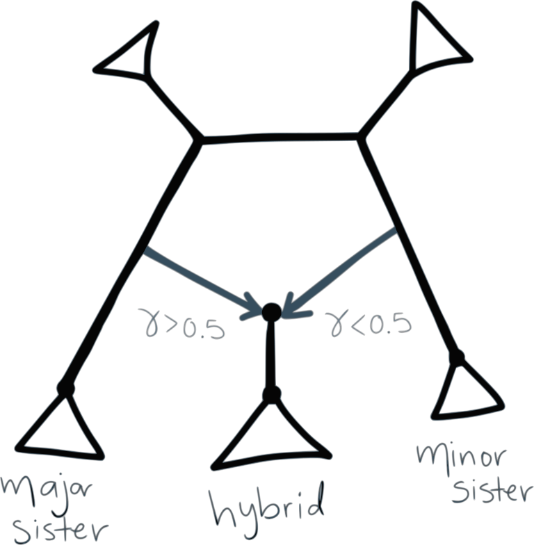
To summarize bootstrap support on networks, we focus on three types of clades:
- hybrid clade: hardwired cluster (descendants) of either hybrid edge
- major sister clade: hardwired cluster of the sibling edge of the major hybrid edge
- minor sister clade: hardwired cluster of the sibling edge of the minor hybrid edge
The following function computes the proportion of times that different clades appear as hybrid, major sister or minor sister in the bootstrap networks:
BSn, BSe, BSc, BSgam, BSedgenum = hybridclades_support(bootnet, net1);
BSnis a table of bootstrap frequencies associated with nodesBSeis a table of bootstrap frequencies associated with edges, andBScdescribes the makeup of all clades.
First, we plot the proportion of times that the major and minor hybrid edges of the best network appear in the bootstrap networks:
plot(net1, edgelabel=BSe[!,[:edge,:BS_hybrid_edge]]);
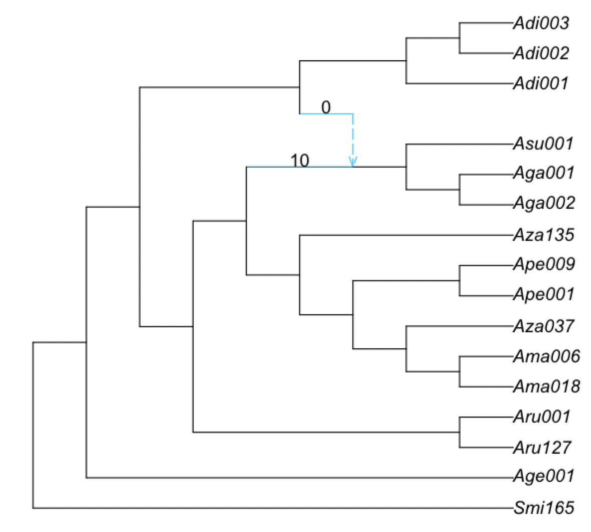
In this case, there are 0% of bootstrap networks that have the major hybrid edge and 0% bootstrap networks that have the minor hybrid edge. Recall that we only ran 10 bootstrap replicates with 1 run each, so the runs have likely not converged in this case.
What do the remaining bootstrap networks have?
julia> BSe
16×8 DataFrame
 Row │ edge     hybrid_clade  hybrid   sister_clade  sister  BS_hybrid_edge  BS_major  BS_minor
     │ Int64?   String        Int64?   String        Int64?  Float64         Float64   Float64
─────┼──────────────────────────────────────────────────────────────────────────────────────────
   1 │      24  H17                15  c_minus10        -10             0.0       0.0       0.0
   2 │      28  H17                15  c_minus3          -3             0.0       0.0       0.0
   3 │ missing  Ape001              9  Ape009            10            30.0      30.0       0.0
   4 │ missing  Ape001              9  H17              -16            30.0       0.0      30.0
   5 │ missing  c_34          missing  Aza135            11            20.0      20.0       0.0
   6 │ missing  c_34          missing  Ape001             9            20.0       0.0      20.0
   7 │ missing  Smi165              2  Age001             3            10.0      10.0       0.0
   8 │ missing  Smi165              2  Ama006             7            10.0       0.0      10.0
   9 │ missing  Adi002             17  Adi003            16            10.0      10.0       0.0
  10 │ missing  Adi002             17  Aru001             4            10.0       0.0      10.0
  11 │ missing  c_35          missing  c_minus8          -8            10.0      10.0       0.0
  12 │ missing  c_35          missing  H17              -16            10.0       0.0      10.0
  13 │ missing  c_minus2           -2  Adi001             1            10.0      10.0       0.0
  14 │ missing  c_minus2           -2  Ama018             6            10.0       0.0      10.0
  15 │ missing  Aru001              4  Aru127             5            10.0      10.0       0.0
  16 │ missing  Aru001              4  Age001             3            10.0       0.0      10.0
We can understand the meaning of each column with ? hybridclade_support in julia.
We can see, for example, that in 30% of the bootstrap networks there is a hybrid edge
from Ape001 to Ape009. Because BS_major is also 30, we conclude that this edge appears as the major hybrid edge in 30% of the bootstrap networks. We note that this edge does not appear in the estimated network (net1) since the column edge is missing.
Sometimes, there is not a taxon name, but a clade, like c_minus8. The information of which clade this represents can be found in the BSc data frame:
julia> BSc
16×18 DataFrame
 Row │ taxa    Adi001  Smi165  Age001  Aru001  Aru127  c_minus8  Ama018  Ama006  Ape001  Ape009  Aza135  H17    c ⋯
     │ String  Bool    Bool    Bool    Bool    Bool    Bool      Bool    Bool    Bool    Bool    Bool    Bool   B ⋯
─────┼─────────────────────────────────────────────────────────────────────────────────────────────────────────────
   1 │ Adi001    true   false   false   false   false     false   false   false   false   false   false  false    ⋯
   2 │ Smi165   false    true   false   false   false     false   false   false   false   false   false  false
   3 │ Age001   false   false    true   false   false     false   false   false   false   false   false  false
   4 │ Aru001   false   false   false    true   false      true   false   false   false   false   false  false
   5 │ Aru127   false   false   false   false    true      true   false   false   false   false   false  false    ⋯
   6 │ Ama018   false   false   false   false   false     false    true   false   false   false   false  false
   7 │ Ama006   false   false   false   false   false     false   false    true   false   false   false  false
   8 │ Aza037   false   false   false   false   false     false   false   false   false   false   false  false
   9 │ Ape001   false   false   false   false   false     false   false   false    true   false   false  false    ⋯
  10 │ Ape009   false   false   false   false   false     false   false   false   false    true   false  false
  11 │ Aza135   false   false   false   false   false     false   false   false   false   false    true  false
  12 │ Asu001   false   false   false   false   false     false   false   false   false   false   false   true
  13 │ Aga002   false   false   false   false   false     false   false   false   false   false   false   true    ⋯
  14 │ Aga001   false   false   false   false   false     false   false   false   false   false   false   true
  15 │ Adi003   false   false   false   false   false     false   false   false   false   false   false  false
  16 │ Adi002   false   false   false   false   false     false   false   false   false   false   false  false
Or specifically:
julia> BSc[!,:taxa][BSc[!,:c_minus8]]
2-element Vector{String}:
 "Aru001"
 "Aru127"
We can look at the estimated network again to find this clade:
and the hybrid clade is:
julia> BSc[!,:taxa][BSc[!,:H17]]
3-element Vector{String}:
 "Asu001"
 "Aga002"
 "Aga001"
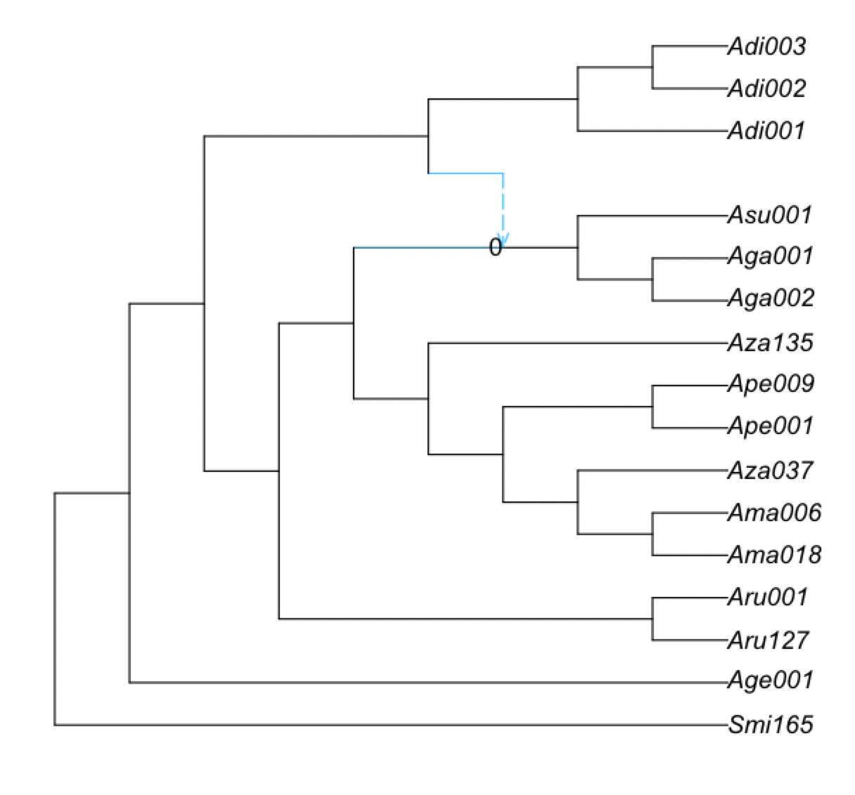
We can also quantity the proportion of the times that the same hybridization event (same hybrid node with same major and minor hybrid edges) appear in the bootstrap networks.
plot(net1, nodelabel=BSn[!,[:hybridnode,:BS_hybrid_samesisters]]);
which in this case (because we did not do enough replicates or enough number of runs) is zero:
We can also plot the bootstrap support for hybrid clades, regardless of their sisters. Here, it is shown on the parent edge of each node with positive hybrid support:
plot(net1, edgelabel=BSn[BSn[!,:BS_hybrid].>0, [:edge,:BS_hybrid]]);