Visualizing the species trees

We have 4 estimated species trees (in results):

full concatenation (RAxML/full-concatenation/triticeae_allindividuals_OneCopyGenes.fasta.raxml.bestTree)
consensus of 10Mb window concatenation trees (folder RAxML/10Mb-concatenation)
supertree (07-supertree.tre)
ASTRAL4 tree (07-individual-species-tree-astral4.tre)

Reproducing Figure 1A

The authors claim that Figure 1A represents both the full concatenation tree and the supertree. Although note that we do not have the same supertree input data: Figure 1: (A) Phylogenetic tree of the Aegilops/Triticum genus. This same topology was obtained by both the ML analysis of 8739 gene alignments concatenation (supermatrix) and the supertree combination of 11,033 individual gene trees.

We will plot the two trees side by side.

In results:

library(ape)

tree1 = read.tree(file="RAxML/full-concatenation/triticeae_allindividuals_OneCopyGenes.fasta.raxml.bestTree")
tree2 = read.tree(file="07-supertree.tre")

tree1 = root(tree1,outgroup="H_vulgare_HVens23", resolve.root=TRUE)
tree2 = root(tree2,outgroup="H_vulgare_HVens23", resolve.root=TRUE)

# Suppose your trees are called tree1 and tree2
# First, ladderize both trees
tree1 <- ladderize(tree1)
tree2 <- ladderize(tree2[[2]])

# Make sure they have the same tip labels
common_tips <- intersect(tree1$tip.label, tree2$tip.label)

length(common_tips)
length(tree1$tip.label)
length(tree2$tip.label)

# Reorder the second tree to match the tip order of the first
tree2 <- reorder.phylo(tree2, order = "cladewise")
tree2 <- rotateConstr(tree2, tree1$tip.label) # rotate to match tree1 tip order

# Plot side by side
par(mfrow = c(1, 2))
plot(tree1, main = "Full concatenation", cex = 0.8)
plot(tree2, main = "Supertree", cex = 0.8)

They don’t look the same. We can calculate the RF distance:

library(phangorn)
RF.dist(tree1, tree2) ## not zero!

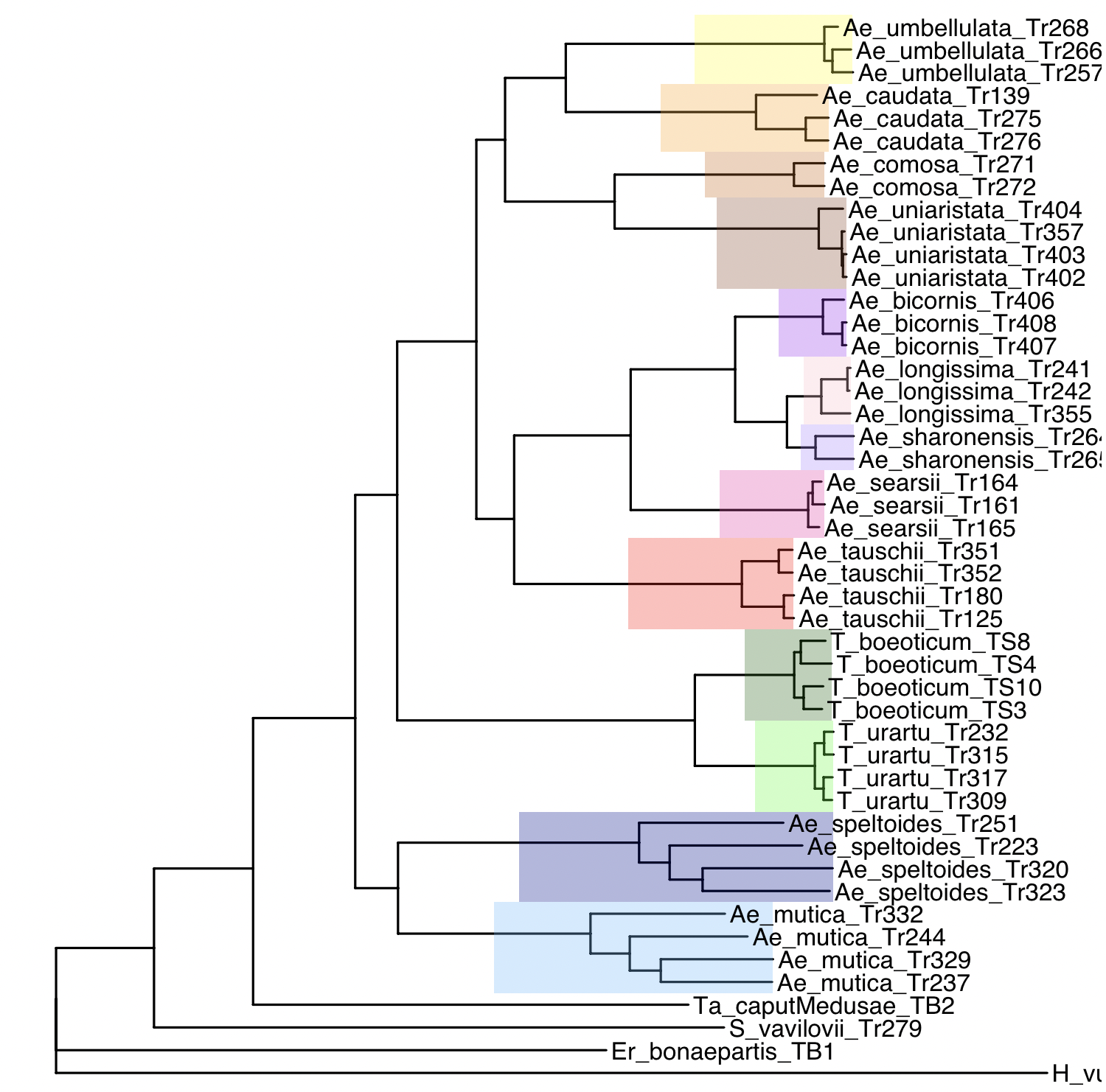
Let’s try to reproduce the edge colors on the full concatenation tree (tree1):

library(ape)
library(ggtree)
library(dplyr)

species_colors <- c(
  "Ae_umbellulata" = "yellow",
  "Ae_caudata" = "orange",
  "Ae_comosa" = "darkorange3",
  "Ae_uniaristata" = "sienna4",
  "Ae_bicornis" = "purple",
  "Ae_longissima" = "pink",
  "Ae_sharonensis" = "mediumpurple1",
  "Ae_searsii" = "maroon2",
  "Ae_tauschii"    = "red",
  "T_boeoticum" = "darkgreen",
  "T_urartu" = "green",
  "Ae_speltoides" = "blue4",
  "Ae_mutica" = "steelblue1"
)

tip_species <- sapply(tree1$tip.label, function(x) {
  parts <- strsplit(x, "_")[[1]]
  paste(parts[1:2], collapse = "_")  # combine first two parts
})
tip_species <- as.factor(tip_species)


p <- ggtree(tree1)

# Loop over species to color clades
for(sp in names(species_colors)) {
  # Get tips belonging to this species
  tips <- tree1$tip.label[tip_species == sp]
  # Get MRCA node
  node <- getMRCA(tree1, tips)
  if(!is.null(node)) {
    p <- p + geom_hilight(node = node, fill = species_colors[sp], alpha = 0.3)
  }
}

# Add tip labels
p <- p + geom_tiplab()
p

We might want to rotate manually some clades to mimic Figure 1A:

p + geom_text2(aes(subset = !isTip, label = node), hjust = -0.3)

We want to rotate the following clades:

p <- ggtree(tree1)

p2 <- rotate(p, node = 55)
p2 <- rotate(p2, node = 62)
p2 <- rotate(p2, node = 50)
p2 <- rotate(p2, node = 49)
p2 <- rotate(p2, node = 69)
p2 <- rotate(p2, node = 83)
p2 <- rotate(p2, node = 88)
p2 <- rotate(p2, node = 71)
p2 <- rotate(p2, node = 74)


for(sp in names(species_colors)) {
  tips <- tree1$tip.label[tip_species == sp]
  node <- getMRCA(tree1, tips)  # this works on phylo object
  if(!is.null(node)) {
    p2 <- p2 + geom_hilight(node = node, fill = species_colors[sp], alpha = 0.3)
  }
}

p2 <- p2 + geom_tiplab()
p2

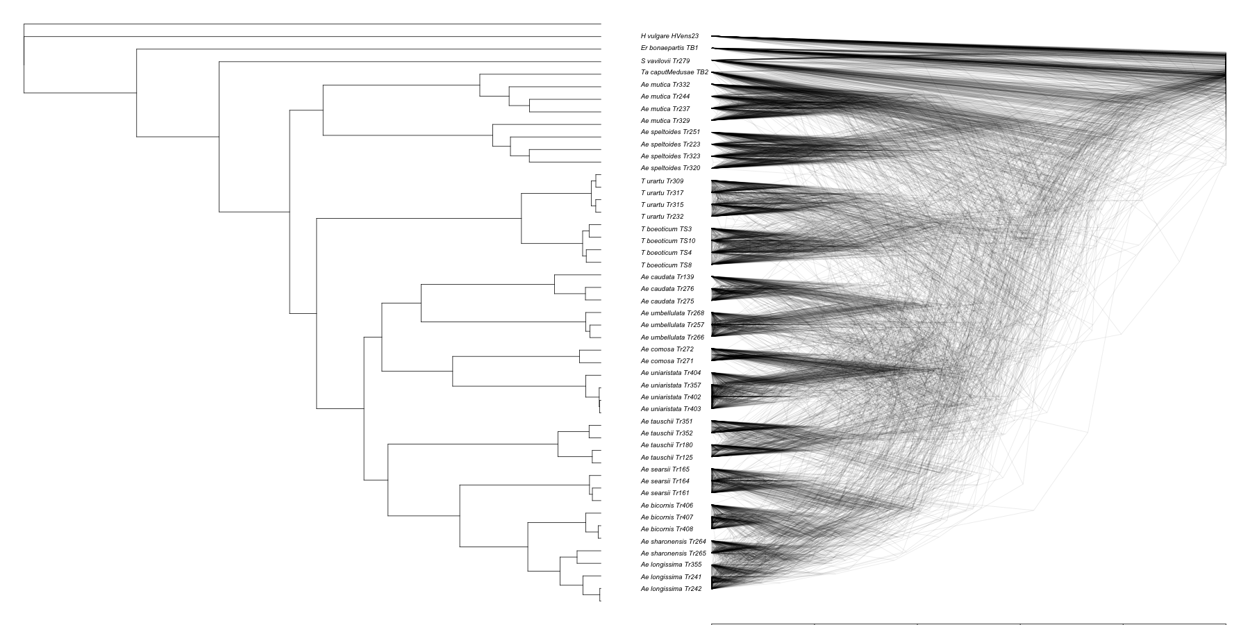
Reproducing Figure 1B

This is almost the same code as in Species tree via concatenation: 10Mb sliding window.

We need to be in the results/RAxML/10Mb-concatenation folder:

library(ape)
library(phangorn)
library(phytools)
library(ggplot2)

tree_files <-list.files(pattern="\\.raxml.bestTree$") #List all .bestTree files. $ ensures the end of the name

trees<- list() # list with all the trees
class(trees)<- "multiPhylo" #make it a multiphylo object for ease of use with other 

i<-1
for(tree_file in tree_files){ ##go thru each file and read the tree
  trees[[i]]<- read.tree(tree_file)
  i<-i+1
}

We need to root all trees in “H_vulgare_HVens23” to reproduce Figure 1(B):

#re-reroot all our gene trees by the respective outgroup
for(i in 1:length(trees)){
  trees[[i]]<- root(trees[[i]],
                         outgroup = "H_vulgare_HVens23",
                         resolve.root=TRUE)
  trees[[i]]<-chronos(trees[[i]]) ## make ultrametric for nicer densitree
}

We will create a consensus parsimony supertree:

st<-superTree(trees)
st<-root(st,"H_vulgare_HVens23",resolve.root = T)

Finally, we plot the same density tree as Figure 1B:

tree1ultra = chronos(tree1)

png(filename="../../../figures/figure1b.png", width = 1800, height = 900, units = "px")
par(mfrow=c(1,2), mar = c(0.1, 0.1, 0.1, 0.1))
plot(tree1ultra, show.tip.label = FALSE)
densiTree(trees,consensus=tree1, direction='leftwards', scaleX=T,type='cladogram', alpha=0.1)
dev.off()

New coalescent-based species tree (ASTRAL4)

We now want to compare the original species tree with the new coalescent-based species tree we inferred with ASTRAL4.

We plot the individual level species tree along with the full concatenation tree (tree1). In results:

tree3 = read.tree(file="07-individual-species-tree-astral4.tre")
tree3 = root(tree3,outgroup="H_vulgare_HVens23", resolve.root=TRUE)

par(mfrow=c(1,2), mar = c(0.1, 0.1, 0.1, 0.1))
plot(tree1)
plot(tree3)

First, we can calculate the RF distance:

> RF.dist(tree1,tree3)
[1] 4 ## not the same tree!

These trees look very similar, but let’s compare the species level tree 07-species-tree-astral4.tre:

tree4 = read.tree(file="07-species-tree-astral4.tre")
tree4 = root(tree4,outgroup="H_vulgare", resolve.root=TRUE)

par(mfrow=c(1,2), mar = c(0.1, 0.1, 0.1, 0.1))
plot(tree1)
plot(tree4)